Michael Hudson’s simple phrase “Debts that can’t be repaid, won’t be repaid” sums up the economic dilemma of our times. This does not involve sanctioning “moral hazard”, since the real moral hazard was in the behavior of the finance sector in creating this debt in the first place. Most of this debt should never have been created. All it did was fund disguised Ponzi schemes that inflated asset values without adding to society’s productivity. The irresponsibility—and Moral Hazard—clearly lay with the lenders rather than the borrowers.
The question we face is not whether to repay this debt, but how to go about not repaying it?
The standard means of reducing debt—personal and corporate bankruptcies for some, slow repayment of debt in depressed economic conditions for others—could have us mired in deleveraging for one and a half decades, given its current rate. That would be one and a half decades where the boost to demand that rising debt should provide—as it finances investment rather than speculation—is absent. Growth is too slow to absorb new entrants into the workforce, innovation is muted, and political unrest rises–with all the social consequences. Just as it did in the Great Depression.
So it is incumbent for society to reduce the debt burden sooner rather than later, so as to reduce the period spent in the damaging process of deleveraging. Pre-Capitalist societies instituted the practice of the Jubilee to escape from similar traps, and debt defaults have been a common experience in the history of Capitalism too. So a prima facie alternative to 15 years of deleveraging is an old-fashioned debt Jubilee.
But a Jubilee in modern Capitalism faces two dilemmas. Firstly, a debt Jubilee would paralyse the financial sector by destroying bank assets. Secondly, in our era of securitized finance, the ownership of debt permeates society in the form of asset based securities (ABS) that generate income streams on which a multitude of non-bank recipients depend. Debt abolition would inevitably destroy both the assets and the income streams of owners of ABSs, most of whom are innocent bystanders to the delusion and fraud that gave us the subprime xrisis, and the myriad fiascos that Wall Street has perpetrated in the 25 years since the 1987 stock market Crash.
We therefore need a way to short-circuit the process of debt-deleveraging, while not destroying the assets of both the banking sector and the members of the non-banking public who purchased ABSs. One feasible means to do this is a “Modern Jubilee”, which could also be described as “Quantitative Easing for the public”.
Quantitative Easing was undertaken in the false belief that this would “kick start” the economy by spurring bank lending. Barack Obama put it:
And although there are a lot of Americans who understandably think that government money would be better spent going directly to families and businesses instead of banks – “Where is our bailout?,” they ask – the truth is that a dollar of capital in a bank can actually result in eight or ten dollars of loans to families and businesses, a multiplier effect that can ultimately lead to a faster pace of economic growth. (Obama 2009)
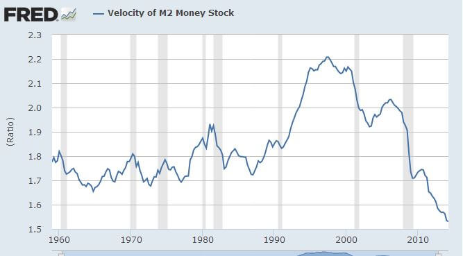
Instead, QE’s main effect was to dramatically increase the idle reserves of the banking sector while the broad money supply stagnated or fell (see figure). There is already too much private sector debt, and neither lenders nor the public want to take on more debt.
A Modern Jubilee would create fiat money in the same way as QE, but would direct that money to the bank accounts of the publicwith the requirement that the first use of this money would be to reduce debt. Debtors whose debt exceeded their injection would have their debt reduced but not eliminated, while at the other extreme, recipients with no debt would receive a cash injection into their deposit accounts.
The broad effects of a Modern Jubilee would be:
Debtors would have their debt level reduced;
Non-debtors would receive a cash injection;
The value of bank assets would remain constant, but the distribution would alter with debt-instruments declining in value and cash assets rising;
Bank income would fall, since debt is an income-earning asset for a bank while cash reserves are not;
The income flows to asset-backed securities would fall, since a substantial proportion of the debt backing such securities would be paid off; and
Members of the public (both individuals and corporations) who owned asset-backed-securities would have increased cash holdings out of which they could spend in lieu of the income stream from ABS’s on which they were previously dependent.
Clearly there are numerous and complex issues to be considered in such a policy:
The scale of money creation needed to have a significant positive impact (without excessive negative effects. [There will obviously be such effects, but their importance should be judged against the alternative of continued deleveraging.]
The mechanics of the money creation process itself (which could replicate those of Quantitative Easing, but may also require changes to regulation prohibitiing Reserve Banks from buying government bonds directly from the Treasury).
The basis on which the funds would be distributed to the public;
Managing bank liquidity problems (since though banks would not be made insolvent by such a policy, they would suffer significant drops in their income streams);
Ensuring that the program did not simply start another asset bubble.
A look at the critique of Gerald Friedman’s analysis of the Sanders economic program. Alan Harvey
Gerald Friedman has taken a hit from the national press and four former chairs of the President’s Council of Economic Advisers. Friedman’s analysis of the economic effects of Bernie Sanders’ economic proposals projected five-plus percent growth rates in the first three years of the program. The CEA chairs lambasted the projections as fantastic. Austan Goolsbee caricatured them as “flying puppies.” The CEA’s attack was immediately challenged by James K. Galbraith and others, who pointed out that Friedman was using standard economic models and concepts, similar to those used at the Congressional Budget Office (CBO) and the CEA itself.
What is it then, standard fare or fantasy economics?
First, a bit of speculation The timing of and absence of detail in the attacks suggest the four CEA chairs responded to the headline numbers without having studied the detail. A second consideration is that Friedman personally supports Hillary Clinton, so the motive for bias is not clear. A third piece of context is the historical record, which shows that five-plus growth is not unprecedented. It was – as Galbraith pointed out – last seen in the mid-1980s during Ronald Reagan’s military build-up accompanied by federal budget deficits far exceeding any in the post-war era prior to Reagan. Note also that the average growth rate under Democratic presidents prior to Barack Obama was 4.2 percent.
Subsequent to Galbraith’s challenge, at least one of the CEA chairs responded with a more detailed view, picking apart Friedman’s methodology. Christina Romer’s review was featured in the New York Times in a piece by Justin Wolfers, though it is not clear that she went as far as Wolfers in her disparagement of Friedman’s methods. Romer criticized Friedman for confusing stocks and flows, suggesting – as I understand it – that the Friedman analysis projected multipliers too far into the future. The multiplier is the increment of new activity produced by an investment or government spending program. The stimulus money spent is income to workers and businesses, who each save some, but spend most, which becomes income to other workers and businesses and results in further spending.
The nature of multipliers is a fascinating and neglected area of economics which we could happily explore at a length not appropriate to this piece. A study done by mainstream economists Mark Zandi and Alan Blinder (conservatively) estimated multipliers that vary from very low – in the .33 area, implying a dollar’s worth of spending produces only thirty-three cents of GDP (for corporate tax cuts) to 1.57 (for infrastructure spending) and 1.74 (for increases in food stamps).
There is additional evidence that multipliers have degraded over time, having been much higher in the 1950s and 1960s. [The role of private debt in eroding multipliers should not be ignored, as it seems to have grown as multipliers declined. The 2008 Bush stimulus plan projected much higher multipliers for tax cuts than was experienced. It is likely that many recipients used the tax cuts to pay down debt rather than spend on into the economy.]
Christina Romer is uniquely qualified to discuss overreach in projections, since she was chair of the CEA during the Obama stimulus period and famously forecast an immediate reduction in unemployment that did not materialize. This failure was seized upon by Republicans to discredit government stimulus entirely. We can, of course, look back and see the economic effects, which were substantial. But because they did not match the projection, the theory of the projectors suffered.
The Obama stimulus (ARRA – American Redevelopment and Recovery Act) was poorly designed, as Joseph Stiglitz pointed out. It was essentially divided in three: (1) Tax breaks for business investment, which has always had a low multiplier, since businesses invest when they see profit, not when they get tax breaks, (2) Subsidies to households, who used them as often for paying down debt as for spending, and (3) Infrastructure spending, which DID have a substantial effect, but with only $200 billion in effective stimulus, the Act fell far short of its promise.
Stimulus also suffered a Larry Summers moment, or moments. “Timely, targeted and temporary” was Summers’ mantra in support of the ineffective Bush effort. As an Obama administration official, Summers was implicated in keeping the ARRA too low. Both Romer and Summers seem to have conflated all multipliers into one.
All of this argues for substantial, strategic and sustained. This point was made repeatedly in the aftermath by academics and public policy analysts in the period after the stimulus. But it was too late, and the political will had been used up.
Romer appears to suggest in the Wolfers piece that multipliers act only during the period of stimulus spending, and she faults Friedman for misunderstanding stocks and flows. It should be obvious, however, that a measure which provokes additional private investment can claim credit for economic activity induced by that additional investment. If Ms. Romer is suggesting otherwise, she is wrong. Investment in equipment and facilities by government contractors and investment in housing by newly employed workers would be among the most likely sources of induced stimulus. Consumer goods producers would have less incentive to invest, since there is large unused capacity already extant, and new investment in the consumer goods sector is as likely to happen in China as in the US, shipping the stimulus offshore.
The Sanders plan IS substantial, strategic and sustained. Infrastructure spending is included, at $200 billion per year (the American Society of Civil Engineers estimates $3.6 trillion is needed by 2020). The health insurance and higher education initiatives benefit for spending that is not offshore-able.
In the end, whether Friedman over-promises as Romer did is open to question. At a minimum his analysis is not fantastic or too far outside the orbit of the mainstream. The political will to get programs of this scale through Congress likely would require the motivation of another crisis like that of 2008. The political nature of the critique is for the reader to decide.
The debate over Greece has an eerie resemblance to the debate over climate change. One side prefers apocalypse to changing its opinion, even in the face of evidence. In fact, as the evidence mounts, the denialists become only the more rigid.
In the case of Greece, the Troika consistently refused to engage the economic issues and evidence. Has austerity worked? Would the course preferred by the Troika result in better results for creditors? Does the hard line improve the prospects for European unity? Have the finance ministers served their respective states, or asked accountability from the banks? No, no, no, no and no. Yet the Neoliberal conviction and prescription is held ever more tightly.
Clearly austerity has not worked and has no prospect of working. Greece is in the condition it finds itself today because it, under pressure from the Troika and after signing the ill-begotten 2012 Agreement, enforced austerity as no other European state has done. The Greek people had five long years, since 2010 to witness that the actual results of attempting to shrink your way to growth are exactly as the Keynesian theory describes.
Clearly creditors are worse off. And acceptance of the Troika line would have only meant default on a larger debt. The best outcome for them (the creditors) would have been to restructure the debt into a form that allowed Greece to recover from the austerity-induced depression and get at least some return. But when the “they” who held the debt became the taxpayers of the states rather than the banks, their financial interests became secondary.
Would the capitulation demanded by Schauebel and the Troika improve prospects for success in the European experiment? That is a laughable proposition. In grim fact, the entire negotiation has been a spectacle of destroying any trust between states and giving lie to any democratic pretense under the EU. It must now be clear that the European Union, the European Central Bank and other institutions are instruments of control, not cooperation. In demonstrating the full power of their bargaining position, the Troika has exposed the depth of their devotion to a top-down Neoliberal agenda.
And there is really no debate on the economic points. The Troika does not deny that austerity was a failure. The Confidence Fairy never came. The privatizations, evisceration of labor protections and cutting of already scanty pensions did not lead anywhere but down. Nor do they deny that it would fail again.
The Troika does not deny that creditors, taxpayers and economies would be better off were the terms of debt made sensible. Nor does it deny that the private banks were bailed out at the expense of European taxpayers. The Troika merely ignores the substance — the economics, the financial realities, and the real sacrifices of the Greeks — and moralizes from a position of no moral authority.
This article is a non-mathematical description of the dynamic economic modeling methods developed by Steve Keen.
In a number of papers and articles Steve Keen describes a mathematical model of the economy built using dynamic modeling techniques. The details of each model vary depending on the title and purpose of the article, but there is a very easily identified core set of components, relationships and methods which can sensibly be described as Steven Keen’s Dynamic Monetary Economic model. I am going to try to give a non-mathematical overview of these core ideas so that anyone who wants to go and read those papers, but does not have much mathematical preparation, can get as much from them as possible.
The use of continuous dynamic modeling is a key feature of Steve’s economic model and a general understanding (albeit non mathematical) of dynamic modeling is necessary to understand it. There are therefore three parts to this article. Firstly a non-mathematical introduction to continuous dynamic modeling in general; secondly a non-mathematical description of the Steve’s dynamic model itself; and lastly a discussion of the graphs which the model creates and which you will see in Steve’s papers.
Part 1. Continuous Dynamic Modeling
A dynamic model describes the behaviour of a system over time. It consist primarily of a number of variables (about 10 in Steve’s case) each having its own modeling formula to control its evolution over the time period being modeled/simulated.
Crucially, and slightly confusingly, in a dynamic model the modeling formulae are not used to ‘set’ the value of their related variable directly but instead are used to change it. After the modeling variables are given an initial value at the beginning of the simulation they continually change at a rate (and direction) determined moment to moment by their controlling formula which take as their inputs the states of some or all the variables in the model including the one it is responsible for.
This focus on change (rather than state) is very significant and is what makes dynamic models so useful for economics because it allows the variables to move much more freely relative to each other so they can do things like cycle and crash.
Although the modeling technique is called ‘Continuous’, computers can only deal in discrete steps. In each tiny step the value of each variable is calculated from its previous value plus the change generated by its modeling formula. The values of each variable at each step are recorded in a table and form the output of the model which can be viewed on line graphs.
Time slicing like this is only an approximation of continuous reality and incurs errors which build up over time. The approximation, however, can be made as accurate as any particular application requires by altering the size of the time steps and the precision of the maths engine used. This ‘approximation’ process was used, in fact, to plot the course of the astronauts to the moon and is still used today for all space navigation involving more than 2 masses.
An important reason that the complexities of dynamic modeling are tolerated is that they can reproduce the cyclic and catastrophic behaviour we see in the economy (and other complex dynamic systems) whereas the static modeling methods used by traditional economists cannot.
At the time traditional economics was developed computers were not around. Economics was forced to develop using static models where external shocks were the only way cyclical and catastrophic events could be explained. After the 1930s depression it was noticed by some that the economy behaved like a dynamic system but the computers were not around to support those theories and so they faded away… until 2007 when it all happened again. And this time we do have computers…
Part 2. Steve Keen’s Dynamic Monetary Model of the Economy
Steve’s models are comprised of two distinct groups of variables: The ‘Financial’ variables and the ‘Production’ variables. The production variables (and their formulae) model economic statistics like wage level, quantities and Price Level. The Financial variables (and their formulae) model money/debt flows in and out of small number of notional banking sector ‘accounts’.
Here are the 5 financial (bank) sector account variables which you will find in most of Steve’s Dynamic Monetary Models : –
Bank Vault. – Representing the banking sector’s monetary assets;
Bank Transactions Account – into which interest from customers is paid and from which bank expenditure are made.
Firm Loan ledger – which is not an account that can store money but a record of the amount of outstanding debt owed by the firm sector to the banking sector
Firm Deposit Account – into which money borrowed by the firm sector is deposited
Household Deposit Account – into which wages are paid.
And here are the 3 ‘production’ variables.
Capital Stock
Price Level
Wage Rate
The modeling formulae for these variables are created by considering a number of real world operations. Here is the list of operations used in Steve’s XYZ paper.
Lending of money from the bank vault to the firms’ deposit accounts.
Payment of interest by firms to the bank’s transactions account.
Payment of interest by the bank on firms’ deposit accounts.
Payment of wages.
Payment of interest on workers’ account balances.
Payment for consumption of the output of firms by bank and workers.
Repayment of loans by firms.
Recording the loans of the existing money stock to firms.
Compounding the debt at the rate of interest on loans.
Recording the payment of interest on loans.
Recording the repayment of loans.
Recording the endogenous creation of new money.
The endogenous creation of new money in response to firms’ investment plans.
Notice there is no relationship between the number of operations and the number of modeling variables. The way these operations are analyzed to create the modeling formulae (one for each variable) is central to Steve’s whole modeling method.
Just as in the real world the ‘books’ of the financial sector must always balance; credits must equal debits etc. To ensure this balance the modeling formulae for the financial variables are derived in the same way that an accountant works:
First the size of each operation is calculated (the amount of money involved). The simplest example of this in Steve’s model is the payment of interest, by the bank, on firms’ deposit accounts. (operation 3 above) The ‘size’ of this operation is simply the rate of deposit interest times the amount of money in the ‘Firm Deposit’ account (fourth item in the list of variables above)
After determining the size of the operation we identify which variables are affected by the operation. In our example, paying interest on firm’s deposits reduces the size of the Bank Transaction account and simultaneously increases the size of the Firm Deposit account by the same amount. This means that the interest calculation appears with a minus sign in the formula controlling the Bank Transaction account and with a plus sign in the formula controlling the Firm Deposit account. It should be apparent that the net result of the operation does not change the amount of money in circulation; it just moves funds around and so accounting integrity has been maintained.
Note that some operations actually do increase the amount of money in circulation (i.e. endogenous money creation) but accounting integrity is still maintained by matching deposits with loan obligations (Firm Loans with Firm Deposits).
This same process is repeated for every operation in the list, gradually building the modeling formula for the financial variables. Because each separate operation is financially credible it can be assumed that the resultant final modeling formula, which are just the sum of all those operations, are also financially credible.
The process by which the controlling formula for the production variables are derived is more arbitrary. Each formula is justified using a separate economic theories; either Steve’s own or other people’s.
Just to give you flavor of what sort of thing we are talking about here is direct quote from the section of the paper dealing with the derivation of the formula controlling the Wage variable
“ … The dynamic disequilibrium price equation is consistent with empirical research into actual price setting behavior (Blinder, 1998; Lee,1998) and is derived analytically in (Keen, 2010) from the equilibrium condition for physical output and the physical demand for commodities. Prices converge to a mark-up over the monetary cost of production, where the mark up factor (1−) is equivalent to the equilibrium workers’ share of real output...”
You should be able to see that this is descriptive economic theory being used to generate a mathematical formula to control a variable in the model.
The last thing to note is that Financial and Production variables interact via their controlling formula which access all variables not just ones in their own category. For instance the size of the wage payments operation (number 4 in the list above) references the Wage Rate variable whose controlling formula was being developed in the direct quote from Steve’s paper above.
And that’s it. We have a set of variables and a formula for each to control how it changes over time. To run the model we simply….
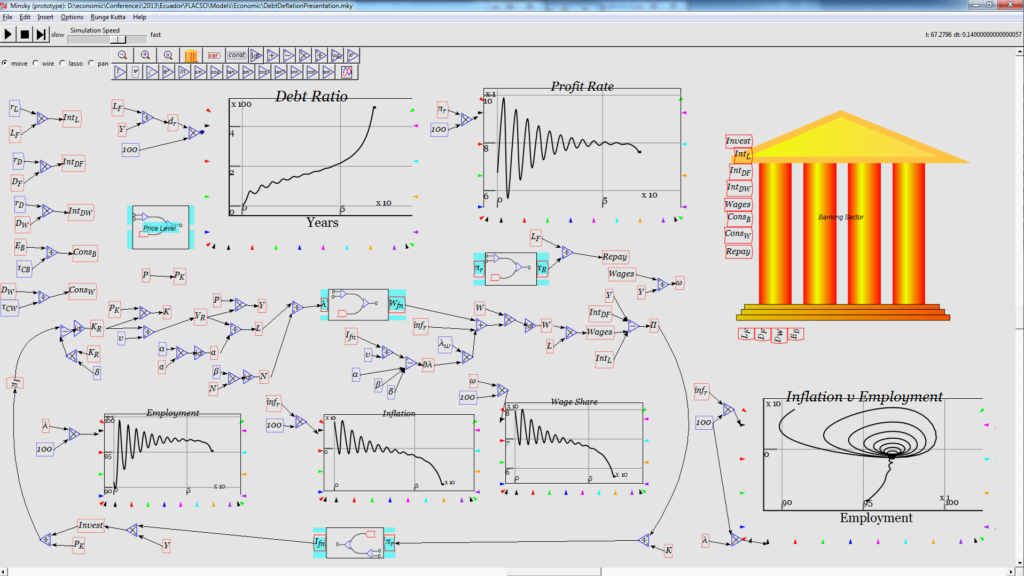
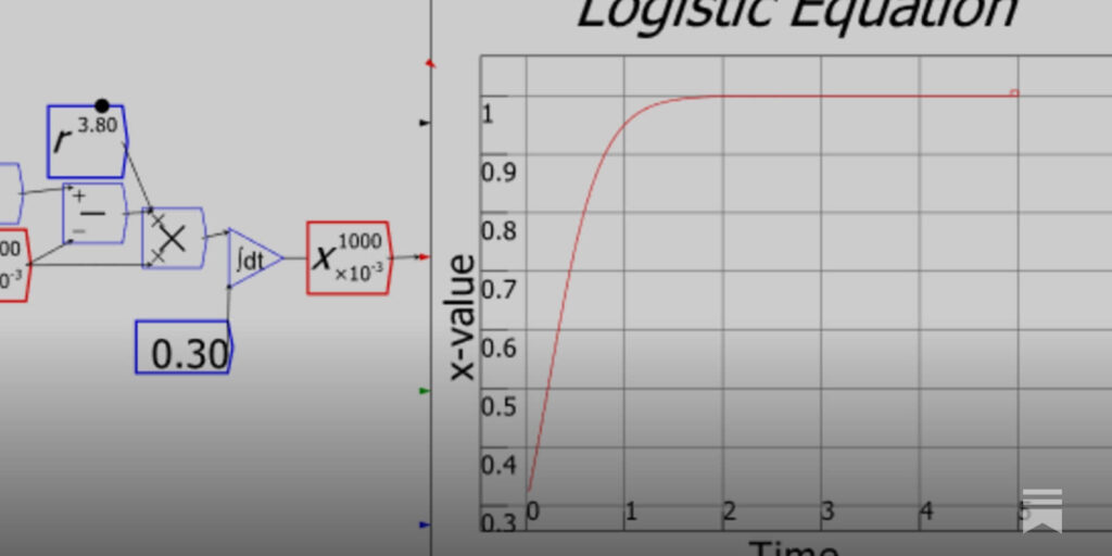
1) Enter the variables and formulae into a Dynamic Modelling package – such as Steve’s own ‘Minsky’
2) Select starting values for the variables (normally set to something other than just zero)
3) Hit the ‘Start Simulation’ button.
Part 3. Graphic output of Steve’s Models
The output of a dynamic model consists of a time series for each of the variables in the model. I.e. a list of values for each variable sampled at regular intervals over the period of the simulation.
It is possible to view this output on a line graph where the X axis represents time, the Y axis represents Money (usually) and each variable has a line displaying its value changing over time. Here is a time series line graph showing the Bank Vault, Firm Loan and Firm Deposit variables from a run of the model. Initially all three variables rise at pretty much the same rate until at about year 50 in the simulation Firm Loans and Deposits collapse whilst the Bank Vault jumps up. This behaviour is exactly what we saw in the great recession. Loans deposits go down as firm investment goes down which causes bank reserves to go up.
As well as simply graphing the model variables we can graph values which are calculated from the variables in the model. Here is a graph of the percentage of GDP earned by Workers, Capitalists and Bankers receive. These are not directly modeled but can be easily calculated from the variables which are in the model.
This chart nicely shows the ‘Great Moderation’ as a series of gradually smaller cycles in GDP share until at around year 50 of the simulation, just as the system seems to settle down, the whole pattern of distribution radically changes: Capitalists and workers both lose share and bankers (ironically) gain it.
Phase Diagrams
Dynamic model output is also commonly viewed as something called a phase diagram which is line graph where each axis represents a single variable from the model. The results are shown as a single line on the graph. The coordinates of each point on the line represent the values of the axis variables at one particular instant.
Here is a fancy looking 3 dimensional phase diagram from one of Steve’s models constructed along the lines described above.
To interpret phase diagrams you have to imagine a dot traveling along the line. It would not be wrong to mark the direction of travel on the line with an arrow although it is normally assumed that this is obvious to an informed viewer. As time progresses the dot moves along the line and its co-ordinates change representing the changing values of the variables they represent. In this case the direction of movement (time) is from the dark purple end of the line at the bottom to the red end at the top.
The circling/spiraling section of the path at the bottom is at the start of the period being modeled. In this early period both ‘debt to output ratio’ and ‘Employment’ go up and down but out sync with each other producing the circling pattern (this is a common pattern in nonlinear dynamic models) During this cyclic phase debt remains low as a proportion of output, but once again at the end of the run it gets out of control and heads upwards rapidly as output collapses.
Conclusions
Clearly this is only the briefest of introductions to Steve’s dynamic models. The key point is that dynamic modeling can reproduce the behaviours we see in the real world as an emergent result whose individual components can each be justified in intuitively satisfying ways relating to day-to-day activities having nothing to do with these emergent results.